Comparing HTFA kernels on real multi-subject fMRI

This tutorial uses a movie-viewing fMRI dataset as a worked example of comparing spatial models. Nilearn’s development_fmri dataset contains children and adults watching Pixar’s short animated film Partly Cloudy. Here we select three adults and fit each participant’s recording with Gaussian (RBF), Laplace, and Mexican-hat kernel shapes, each with one or two components per factor. A kernel specifies a factor’s spatial profile around a center; a mixture combines several spatial lobes into one factor with a shared time course. Every candidate uses these same recordings. The question is which candidate reconstructs this dataset best; the comparison does not establish a population ranking of kernels.

Movie viewing is an illustrative source of multi-subject images, not a requirement of kernel comparison. The same comparison can be applied to other task or resting-state data when the observations, masks, preprocessing, and evaluation protocol are held fixed across candidates.

Each recording contains 168 brain volumes acquired 2 seconds apart. The comparison fixes K=15 and uses the same subjects, preprocessing, all frames, and full voxel masks throughout. We try two starts per candidate, selecting by full-data RSS. Optimization uses 3000 voxels per subject; scoring uses every voxel. Candidate runtime and convergence are recorded. More components enlarge the model class, but local optimization and regularization need not produce monotonically improving fits.

The AIC/AICc/BIC values below use the nominal conditional Gaussian convention explained in Tutorial 14; they are not hierarchical marginal likelihoods. Real fMRI violates independent residual assumptions. The complete run refits locally and may take several minutes; downloading is cached.

# Install htfa from PyPI if needed (for example on Colab).
try:
    import htfa  # noqa: F401
except ImportError:
    %pip install -q htfa

import time
import warnings

import numpy as np

import htfa
from htfa.io import Subject
from htfa.stats import parameter_count, reconstruction_statistics
from htfa.tfa import standardize_data

pd = htfa.require("pandas")
plt = htfa.require("matplotlib.pyplot")

data = htfa.datasets.fetch_development_fmri(n_subjects=3)
subjects = [Subject(x, r) for x, r in zip(data.data, data.coords, strict=True)]
print("Subjects:", data.subject_ids)
print("Shapes:", [x.shape for x in data.data])
settings = dict(
    K=15,
    template_update="fixed",
    max_global_iter=25,
    max_voxels=3000,
    init="ncorr",
    n_jobs=3,
)
print(settings)

Subjects: ['sub-pixar123', 'sub-pixar124', 'sub-pixar125']
Shapes: [(25079, 168), (23726, 168), (26739, 168)]
{'K': 15, 'template_update': 'fixed', 'max_global_iter': 25, 'max_voxels': 3000, 'init': 'ncorr', 'n_jobs': 3}

records, results, attempts = [], {}, []
for kernel in ("rbf", "laplace", "mexican_hat"):
    for components in (1, 2):
        label = f"{kernel}, M={components}"
        best = None
        started = time.perf_counter()
        for seed in (0, 1):
            with warnings.catch_warnings(record=True) as caught:
                warnings.simplefilter("always")
                model = htfa.HTFA(
                    **settings,
                    kernel=kernel,
                    n_components=components,
                    random_state=seed,
                ).fit(data.data, data.coords)
            result = htfa.HTFAResults(model, subjects)
            score = reconstruction_statistics(result)
            attempts.append(
                dict(
                    candidate=label,
                    seed=seed,
                    rss=score.rss,
                    iterations=model.n_iter_,
                    reason=model.converged_reason_,
                    warnings="; ".join(str(w.message) for w in caught),
                )
            )
            if best is None or score.rss < best[0].rss:
                best = score, result, seed
        score, result, seed = best
        results[label] = result
        records.append(
            dict(
                candidate=label,
                seed=seed,
                seconds=time.perf_counter() - started,
                **parameter_count(result),
                **score.to_dict(),
            )
        )
        print(label, "R²", round(score.r2, 4), "BIC", round(score.bic), flush=True)
table = pd.DataFrame(records).set_index("candidate")
for name in ("aic", "aicc", "bic"):
    table["delta_" + name] = table[name] - table[name].min()
table[
    [
        "r2",
        "spatial",
        "temporal",
        "n_parameters",
        "delta_aic",
        "delta_aicc",
        "delta_bic",
        "seconds",
    ]
]

rbf, M=1 R² 0.0541 BIC 35437009
rbf, M=2 R² 0.0573 BIC 35398391
laplace, M=1 R² 0.0531 BIC 35450219
laplace, M=2 R² 0.0562 BIC 35413071
mexican_hat, M=1 R² 0.0538 BIC 35440961
mexican_hat, M=2 R² 0.0568 BIC 35405264

	r2	spatial	temporal	n_parameters	delta_aic	delta_aicc	delta_bic	seconds
candidate
rbf, M=1	0.054125	180	7560	7741	41847.430115	41846.872638	38617.232347	12.070661
rbf, M=2	0.057273	405	7560	7966	0.000000	0.000000	0.000000	45.435278
laplace, M=1	0.053140	180	7560	7741	55058.199472	55057.641994	51828.001703	16.174762
laplace, M=2	0.056182	405	7560	7966	14679.207184	14679.207184	14679.207184	50.075899
mexican_hat, M=1	0.053831	180	7560	7741	45799.958603	45799.401125	42569.760835	14.471393
mexican_hat, M=2	0.056762	405	7560	7966	6872.209722	6872.209722	6872.209722	44.860440

Fit quality and penalty

R² favors smaller residuals; ΔIC is relative to the best candidate under each criterion (zero is best). Temporal parameter counts are identical because K and T are fixed, while component counts change the spatial budget. A large ΔBIC here is not calibrated evidence under residual dependence.

fig, axes = plt.subplots(1, 2, figsize=(12, 4))
table.r2.plot.bar(ax=axes[0], title="Full-data reconstruction R²")
table[["delta_aic", "delta_bic"]].plot.bar(
    ax=axes[1], title="Nominal conditional criteria (lower is better)"
)
plt.tight_layout()
plt.show()
print("Highest R²:", table.r2.idxmax())
print("Lowest nominal AIC:", table.aic.idxmin())
print("Lowest nominal BIC:", table.bic.idxmin())
pd.DataFrame(attempts)[["candidate", "seed", "rss", "iterations", "reason"]]

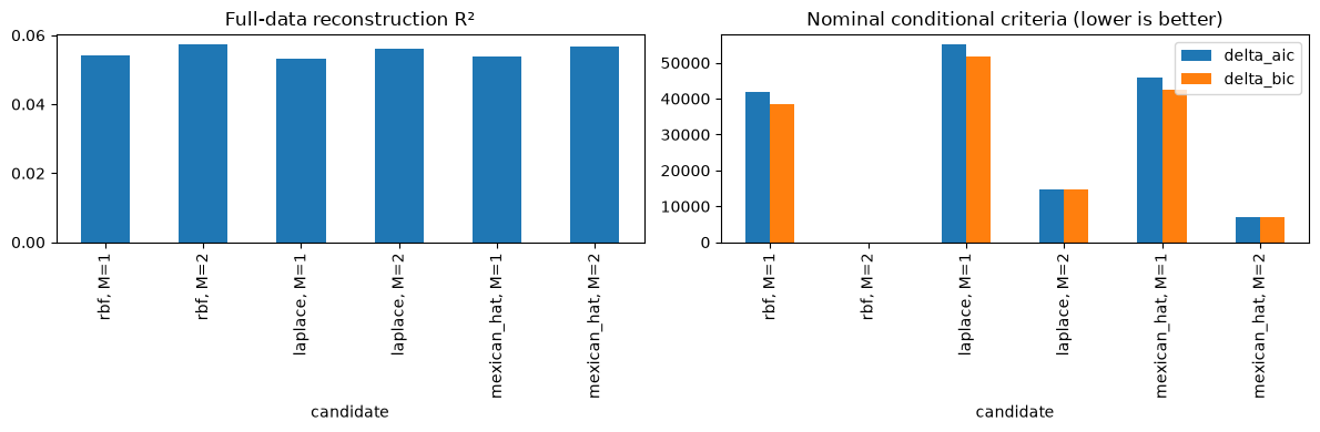
Highest R²: rbf, M=2
Lowest nominal AIC: rbf, M=2
Lowest nominal BIC: rbf, M=2

	candidate	seed	rss	iterations	reason
0	rbf, M=1	0	1.200865e+07	7	plateau
1	rbf, M=1	1	1.200446e+07	6	threshold
2	rbf, M=2	0	1.196899e+07	9	plateau
3	rbf, M=2	1	1.196452e+07	13	plateau
4	laplace, M=1	0	1.201780e+07	8	plateau
5	laplace, M=1	1	1.201697e+07	8	plateau
6	laplace, M=2	0	1.197955e+07	8	plateau
7	laplace, M=2	1	1.197837e+07	7	plateau
8	mexican_hat, M=1	0	1.200820e+07	11	plateau
9	mexican_hat, M=1	1	1.201406e+07	6	plateau
10	mexican_hat, M=2	0	1.197100e+07	13	plateau
11	mexican_hat, M=2	1	1.197143e+07	9	plateau

Example reconstructed frames

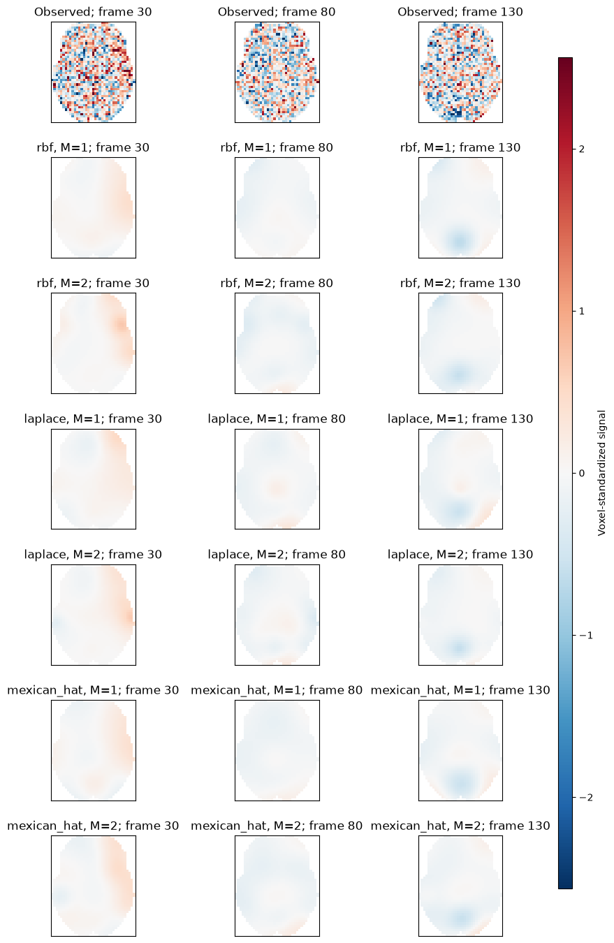
The displayed examples use the first selected participant (subject=0) at acquisition frames 30, 80, and 130. These are illustrative snapshots of reconstruction at different points in the recording, not annotated movie events or selected experimental conditions. Each row uses the same axial slice nearest z=0 in Montreal Neurological Institute (MNI) coordinates, the common anatomical coordinate system of the images. Every panel shares the same symmetric scale in voxel-standardized units, including the observed frames; no reconstruction is independently rescaled. Outside-mask locations are blank. These examples show spatial reconstruction, not forecast accuracy.

frames = [30, 80, 130]
coords = data.coords[0]
z = np.unique(coords[:, 2])[np.argmin(abs(np.unique(coords[:, 2])))]
keep = coords[:, 2] == z
xx, ix = np.unique(coords[keep, 0], return_inverse=True)
yy, iy = np.unique(coords[keep, 1], return_inverse=True)
observed = standardize_data(data.data[0], True)
arrays = {
    "Observed": observed,
    **{name: res.reconstruct(0) for name, res in results.items()},
}
limit = np.percentile(abs(observed[keep][:, frames]), 99)
fig, axes = plt.subplots(len(arrays), len(frames), figsize=(10, 17))
for row, (label, values) in enumerate(arrays.items()):
    for col, frame in enumerate(frames):
        plane = np.full((len(yy), len(xx)), np.nan)
        plane[iy, ix] = values[keep, frame]
        im = axes[row, col].imshow(
            plane,
            origin="lower",
            cmap="RdBu_r",
            vmin=-limit,
            vmax=limit,
            extent=[xx.min(), xx.max(), yy.min(), yy.max()],
        )
        axes[row, col].set_title(f"{label}; frame {frame}")
        axes[row, col].set_xticks([])
        axes[row, col].set_yticks([])
fig.subplots_adjust(right=0.87, hspace=0.35)
fig.colorbar(
    im, cax=fig.add_axes([0.9, 0.15, 0.02, 0.7]), label="Voxel-standardized signal"
)
plt.show()

Scope of the conclusion

The printed winners answer a descriptive question about these three participants, K=15 and this optimization budget. A penalized winner can differ from the R² winner. The figures expose what additional components capture rather than treating a scalar rank as the whole result. Check the start/convergence table before interpreting small differences; reaching the iteration limit is not proof of an optimum.

This comparison is in-sample and uses full-run preprocessing. It does not establish held-out performance, independent-subject generalization or a universally best kernel. A subsequent blocked validation study should refit preprocessing and HTFA within each training split and keep the evaluation mask identical across candidates.

Reading the results

The printed table identifies the best candidate under R² and each nominal information criterion. Inspect the differences across starts and their convergence reasons alongside the scores. More mixture parameters increase the complexity penalty; the residual reduction determines whether a mixture ranks above its single-component counterpart. Continuing a regularized hierarchical fit need not decrease full-data RSS monotonically because the optimization objective includes priors. Correlated residuals mean that large ΔIC magnitudes do not imply calibrated certainty.