Word ↔ brain decoding with HTFA (Mitchell et al., 2008)

Mitchell et al. (2008, Science 320:1191) recorded fMRI while nine participants viewed 60 concrete nouns (12 categories of 5 words, e.g. dog, hammer, house), each with a line drawing, six times each. Their study asks whether word features can predict brain activity for nouns omitted from training. Here the dataset is an illustrative supervised-learning example: HTFA supplies a common set of spatial factors, and regression maps between their weights and numerical word representations (embeddings). The two tasks below use modern sentence embeddings rather than the original verb co-occurrence features, and a different evaluation protocol, so this is not a reproduction of the original study:

1. brain prediction: word embedding → HTFA weights → predicted image of the held-out word in the held-out participant’s voxels;

2. word decoding: the held-out participant’s real HTFA weights → predicted embedding → which of the 60 nouns?

Both mappings are learned on the other 8 participants and never see the held-out word in any participant. The held-out participant’s weights and images are z-scored and centered with the mean and SD of its own 59 training words, so that fold-specific normalization excludes the held-out word. Initial voxel standardization and the unsupervised HTFA fit use the complete runs: this is transductive template evaluation, not a fully held-out preprocessing pipeline.

Run time. By default the notebook loads checksum-verified saved fits, embeddings and permutation nulls, then recomputes the decoding and figures. The cells describe the cached assets and report timing for computations performed during execution. REFIT, RECOMPUTE_EMBEDDINGS and RECOMPUTE_NULL enable recomputation; refitting and permutation testing can take substantially longer. Downloads are cached.

Data. The nine data-science-P*.mat files (about 60 MB each) come from the dataset page and are cached in ~/.cache/htfa/mitchell2008 (or $HTFA_DATA/mitchell2008). The next cell installs htfa from PyPI if it is not installed; matplotlib, nilearn, hypertools and sentence-transformers (the tutorials extra) are installed the first time they are used.

The transferable idea is to use spatial factor weights as features or prediction targets in a separate model. Nouns, sentence embeddings, and this particular participant/word split define the worked example; HTFA itself does not require language stimuli or provide a word-decoding model.

# Install htfa if it is missing (for example on Colab); other packages
# install themselves the first time they are needed.
try:
    import htfa  # noqa: F401
except ImportError:
    %pip install -q htfa

1. Download

Each file holds one participant: 360 trial images (60 nouns × 6 presentations). Per the dataset documentation, each trial image is the mean percent signal change 4 to 8 s after stimulus onset; the data were corrected for slice timing, motion and linear trend, high-pass filtered, normalized to MNI space with SPM and resampled to 3 × 3 × 6 mm voxels.

import hashlib
import json
import os
import time
import urllib.request
import warnings
from pathlib import Path

import nibabel as nib
import numpy as np
import scipy.io
from joblib import Parallel, delayed
from sklearn.exceptions import ConvergenceWarning

import htfa
from htfa.tfa import standardize_data

t_notebook = time.perf_counter()
plt = htfa.require("matplotlib.pyplot")
datasets = htfa.require("nilearn.datasets")
plotting = htfa.require("nilearn.plotting")
print("htfa", htfa.__version__)
print("CPUs:", os.cpu_count())

URL = "https://www.cs.cmu.edu/afs/cs/project/theo-73/www/science2008"
DATA_HOME = Path(os.environ.get("HTFA_DATA", Path.home() / ".cache" / "htfa"))
CACHE = DATA_HOME / "mitchell2008"
CACHE.mkdir(parents=True, exist_ok=True)


def fetch(name):
    """Download one file of the dataset into CACHE (once) and return its path."""
    path = CACHE / name
    if not path.exists():
        tmp = path.with_suffix(".part")
        urllib.request.urlretrieve(f"{URL}/{name}", tmp)
        tmp.rename(path)
    return path


t0 = time.perf_counter()
files = [fetch(f"data-science-P{p}.mat") for p in range(1, 10)]
print(
    f"{len(files)} files, {sum(f.stat().st_size for f in files) / 1e6:.0f} MB, "
    f"{time.perf_counter() - t0:.0f} s (0 s when already cached)"
)

htfa 0.1.0
CPUs: 12
9 files, 538 MB, 0 s (0 s when already cached)

2. Load the trials and the voxel coordinates

meta.colToCoord gives the (1-based) voxel indices of every column of data. The dataset’s functions.tar.gz converts them to MNI millimetres with a fixed matrix (get_mni_coordinates.m), copied below; its in-plane step is 3.125 mm. Each participant has a different set of voxels, which HTFA allows: the factors are functions of MNI coordinates, not of voxel indices.

# get_mni_coordinates.m from the dataset's functions.tar.gz: 1-based voxel
# indices (i, j, k) -> MNI millimetres
VOX_TO_MNI = np.array(
    [
        [-3.125, 0.0, 0.0, 81.25],
        [0.0, 3.125, 0.0, -115.625],
        [0.0, 0.0, 6.0, -54.0],
        [0.0, 0.0, 0.0, 1.0],
    ]
)
AFFINE = VOX_TO_MNI.copy()  # the same map for 0-based indices, for NIfTI images
AFFINE[:3, 3] += VOX_TO_MNI[:3, :3].sum(axis=1)


def load_participant(path):
    m = scipy.io.loadmat(path)
    meta, info = m["meta"][0, 0], m["info"][0]
    X = np.vstack([trial[0].ravel() for trial in m["data"][:, 0]]).T  # (V, 360)
    ijk = meta["colToCoord"].astype(int) - 1  # 0-based voxel indices
    coords = nib.affines.apply_affine(AFFINE, ijk)
    words = np.array([str(t["word"][0]) for t in info])
    cats = np.array([str(t["cond"][0]) for t in info])
    shape = tuple(int(meta[d][0, 0]) for d in ("dimx", "dimy", "dimz"))
    return dict(X=X, coords=coords, ijk=ijk, words=words, cats=cats, shape=shape)


subjects = [load_participant(f) for f in files]
# vocabulary: the 60 nouns, sorted by category and then alphabetically
vocab_pairs = sorted(set(zip(subjects[0]["cats"], subjects[0]["words"], strict=True)))
vocab = np.array([w for _, w in vocab_pairs])
vocab_cats = np.array([c for c, _ in vocab_pairs])
for p, s in enumerate(subjects, 1):
    counts = {w: int((s["words"] == w).sum()) for w in vocab}
    assert set(s["words"]) == set(vocab) and set(counts.values()) == {6}, p
    assert set(zip(s["cats"], s["words"], strict=True)) == set(vocab_pairs), p
print("voxels per participant:", [s["X"].shape[0] for s in subjects])
print("trials per participant:", {s["X"].shape[1] for s in subjects})
print("grid:", subjects[0]["shape"], "| categories:", len(set(vocab_cats)))
print("first 12 trials of P1:", list(subjects[0]["words"][:12]))

voxels per participant: [21764, 21253, 20651, 20395, 20601, 19919, 19750, 20082, 21344]
trials per participant: {360}
grid: (51, 61, 23) | categories: 12
first 12 trials of P1: [np.str_('refrigerator'), np.str_('barn'), np.str_('bell'), np.str_('key'), np.str_('window'), np.str_('screwdriver'), np.str_('church'), np.str_('desk'), np.str_('cow'), np.str_('knife'), np.str_('train'), np.str_('beetle')]

Check: do the coordinates land in the brain?

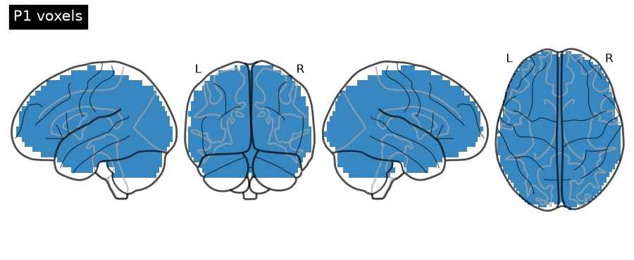
If the matrix is right, the voxels should fill the MNI brain. Between 99.1% and 99.3% of each participant’s voxels fall inside nilearn’s MNI152 brain mask, and the coordinates span about -69 to 72 mm (x), -106 to 72 mm (y) and -48 to 78 mm (z). The glass brain shows P1’s voxels.

def to_nifti(values, s):
    """Put a vector of voxel values of participant s into a 3D NIfTI image."""
    vol = np.zeros(subjects[s]["shape"])
    i, j, k = subjects[s]["ijk"].T
    vol[i, j, k] = values
    return nib.Nifti1Image(vol, AFFINE)


mni_mask = datasets.load_mni152_brain_mask()
inv = np.linalg.inv(mni_mask.affine)
mask_data = mni_mask.get_fdata() > 0
for p, s in enumerate(subjects, 1):
    idx = np.rint(nib.affines.apply_affine(inv, s["coords"])).astype(int)
    inside = mask_data[tuple(idx.T)].mean()
    lo, hi = s["coords"].min(0), s["coords"].max(0)
    print(
        f"P{p}: {inside:.1%} of voxels inside the MNI152 brain mask; "
        f"x {lo[0]:.0f}..{hi[0]:.0f}, y {lo[1]:.0f}..{hi[1]:.0f}, "
        f"z {lo[2]:.0f}..{hi[2]:.0f} mm"
    )
plotting.plot_glass_brain(
    to_nifti(np.ones(len(subjects[0]["coords"])), 0),
    display_mode="lyrz",
    cmap="Blues",
    vmin=0,
    vmax=1.5,
    colorbar=False,
    title="P1 voxels",
)
plt.show()

P1: 99.1% of voxels inside the MNI152 brain mask; x -69..69, y -106..72, z -48..78 mm
P2: 99.1% of voxels inside the MNI152 brain mask; x -69..69, y -103..72, z -42..72 mm
P3: 99.3% of voxels inside the MNI152 brain mask; x -69..69, y -103..72, z -48..78 mm
P4: 99.1% of voxels inside the MNI152 brain mask; x -69..69, y -103..72, z -42..72 mm
P5: 99.3% of voxels inside the MNI152 brain mask; x -69..69, y -106..69, z -48..78 mm
P6: 99.3% of voxels inside the MNI152 brain mask; x -69..69, y -106..72, z -36..72 mm
P7: 99.1% of voxels inside the MNI152 brain mask; x -69..72, y -106..72, z -36..72 mm
P8: 99.3% of voxels inside the MNI152 brain mask; x -69..69, y -106..72, z -48..78 mm
P9: 99.3% of voxels inside the MNI152 brain mask; x -69..69, y -103..72, z -48..72 mm

3. Fit HTFA (K = 100)

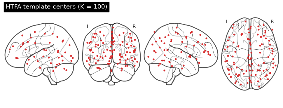
The fit is unsupervised: it sees the 360 trial images of each participant, not the word labels. Each iteration solves for the centers and widths on a random subset of at most 10,000 voxels (max_voxels=10000; all 360 trials); the weights always use all voxels (see the Performance page). init='ncorr' uses one start per participant instead of the three of init='auto'. By default (REFIT = False) the cell downloads a saved copy of this fit with htfa.datasets.fetch_tutorial_fit from the tutorial-data-v1 data release of the htfa repository, checks its SHA-256 and loads it with np.load(..., allow_pickle=False); the printed lines describe the fitting settings. REFIT = True fits it again (the result is not cached).

The cell reports the iteration count and convergence status. Reaching the iteration limit does not establish convergence.

Evaluation scope. This template is fitted with all nine participants, including the one held out below; the held-out participant’s word labels are never used, but its unlabelled images contribute to the template.

# Fit from scratch (True), or download
# the saved fit made with the same settings (False, the default; 2.5 MB).
REFIT = False
NAME = "mitchell2008_K100"
Xs = [s["X"] for s in subjects]
Rs = [s["coords"] for s in subjects]
fit_kwargs = dict(
    K=100, max_voxels=10000, init="ncorr", backend="numpy", n_jobs=3, random_state=0
)


if REFIT:
    t0 = time.perf_counter()
    with warnings.catch_warnings(record=True) as caught:
        warnings.simplefilter("always", ConvergenceWarning)
        model = htfa.fit(Xs, coords=Rs, **fit_kwargs).model
    print(f"fit time: {time.perf_counter() - t0:.0f} s")
    print("warnings:", sorted({w.category.__name__ for w in caught}))
else:
    fit = htfa.datasets.fetch_tutorial_fit(NAME)
    assert json.loads(str(fit["settings"])) == fit_kwargs, fit["settings"]
    assert list(fit["n_voxels"]) == [X.shape[0] for X in Xs]
    model = htfa.HTFA(**fit_kwargs)  # filled with the saved estimates
    model.centers_ = list(fit["centers"])
    model.widths_ = list(fit["widths"])
    model.weights_ = list(fit["weights"])
    model.global_centers_ = fit["global_centers"]
    model.global_widths_ = fit["global_widths"]
    model.n_iter_ = int(fit["n_iter"])
    model.converged_ = bool(fit["converged"])
    print(f"saved fit: htfa.datasets.fetch_tutorial_fit({NAME!r}), SHA-256 checked")
    print("settings:", fit["settings"])
res = htfa.HTFAResults(model, htfa.load(Xs, coords=Rs))
print("global iterations:", model.n_iter_, "| converged:", model.converged_)
print("weights per participant:", {w.shape for w in res.weights})
plotting.plot_connectome(
    np.zeros((100, 100)),
    res.global_centers,
    node_size=12,
    node_color="tab:red",
    display_mode="lyrz",
    colorbar=False,
    title="HTFA template centers (K = 100)",
)
plt.show()

saved fit: htfa.datasets.fetch_tutorial_fit('mitchell2008_K100'), SHA-256 checked
settings: {"K": 100, "max_voxels": 10000, "init": "ncorr", "backend": "numpy", "n_jobs": 3, "random_state": 0}
global iterations: 10 | converged: False
weights per participant: {(100, 360)}

4. One weight vector per word

For each participant, the 6 presentations of each noun are averaged: the weights give a (60, K) matrix per participant, and the per-voxel z-scored data (the same z-scoring the fit applied) give a (60, V) matrix of word images. The mean r(F w, word image) line measures how well K = 100 factors can represent a word image when the weights are known.

The template is a compromise between participants. The next cell reports how often local factors are nearest to their matched template factor, their displacement, and template spacing. These diagnostics should be read alongside the reconstruction scores rather than assuming perfect anatomical correspondence.

# Per-word means: 6 presentations -> one weight vector (K) and one image (V)
Ws, imgs = [], []
for s, w in zip(subjects, res.weights, strict=True):
    Z = standardize_data(s["X"], "auto")  # the per-voxel z-scoring the fit used
    Ws.append(np.stack([w[:, s["words"] == v].mean(axis=1) for v in vocab]))
    imgs.append(np.stack([Z[:, s["words"] == v].mean(axis=1) for v in vocab]))
Fs = [res.factors(s) for s in range(len(subjects))]
print("per-word weights:", Ws[0].shape, "| per-word images of P1:", imgs[0].shape)

# How much of the per-word images the K = 100 factors can represent at all
fit_r = [
    np.mean([np.corrcoef(F @ W[i], img[i])[0, 1] for i in range(60)])
    for F, W, img in zip(Fs, Ws, imgs, strict=True)
]
print("mean r(F w, word image) per participant:", np.round(fit_r, 2))

# How far each participant's local factors moved from the template
G = model.global_centers_
own, shift = [], []
for c in model.centers_:
    d = np.linalg.norm(c[:, None] - G[None], axis=2)  # (K local, K template)
    own.append(d.argmin(1) == np.arange(len(G)))
    shift.append(np.diag(d))
dG = np.linalg.norm(G[:, None] - G[None], axis=2)
np.fill_diagonal(dG, np.inf)
print(
    f"local factors nearest to their own template factor: {np.mean(own):.1%} "
    f"of {np.size(own)}; median distance to it {np.median(shift):.1f} mm; "
    f"median template nearest-neighbour spacing {np.median(dG.min(1)):.1f} mm"
)

per-word weights: (60, 100) | per-word images of P1: (60, 21764)
mean r(F w, word image) per participant: [0.44 0.39 0.42 0.39 0.47 0.43 0.43 0.43 0.43]
local factors nearest to their own template factor: 81.1% of 900; median distance to it 8.9 mm; median template nearest-neighbour spacing 18.6 mm

5. Word embeddings

Model. Qwen/Qwen3-Embedding-0.6B is an Apache-2.0 sentence-transformer model with 1024-dimensional output. The cached embeddings use revision 97b0c614be4d77ee51c0cef4e5f07c00f9eb65b3. The model is available without an access token and can run on CPU or a Colab runtime.

HyperTools. HyperTools 1.1 provides hypertools.tools.format_data with a sentence-transformers model ID as vectorizer. semantic=None skips topic modeling, and ppca=False preserves all embedding dimensions. Each input consists of one noun, with no instruction prefix or surrounding sentence.

Cached and recomputed embeddings. With RECOMPUTE_EMBEDDINGS=False, htfa.datasets.fetch_tutorial_fit loads the embeddings used by the cached permutation null. With True, the cell computes embeddings from the model’s current revision and numerical precision. Recomputed embeddings can differ, so they require a corresponding recomputed null.

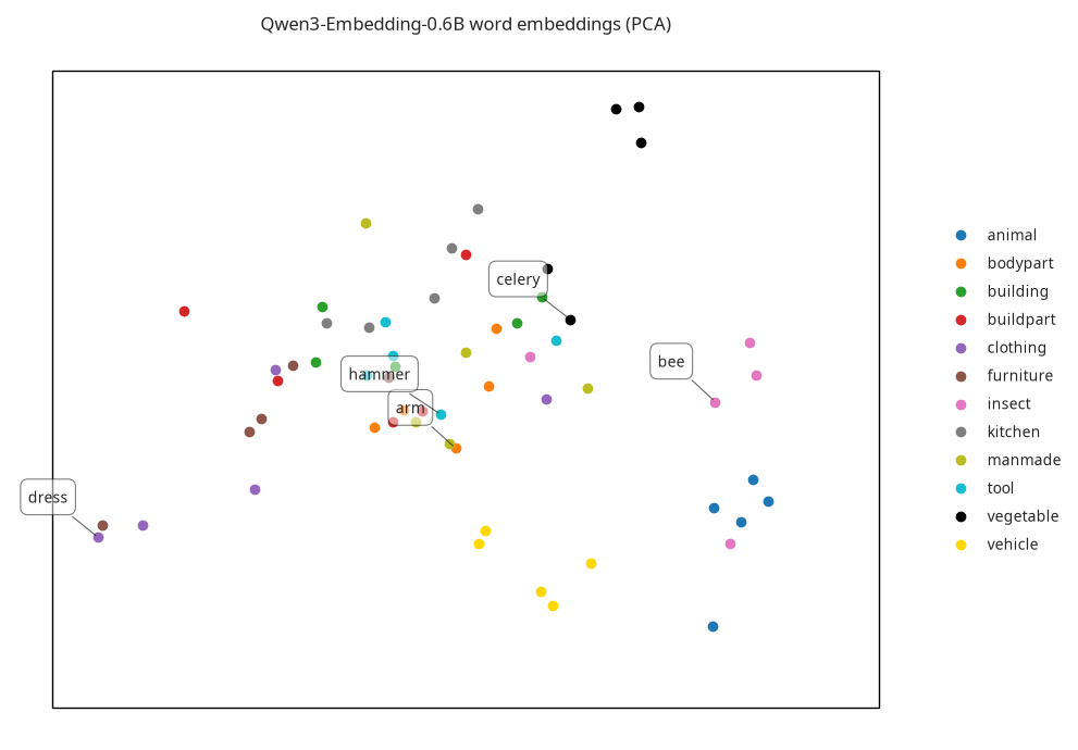
The cell compares correlations within and between noun categories, and reports nearest neighbours for three example nouns. hypertools.plot projects the embeddings to two dimensions with PCA, colors them by category (hue), and labels selected nouns (labels). Its return value is a matplotlib Figure, which supports methods such as savefig. The display is a projection of lexical and semantic similarity, not a test of decoding performance.

import logging  # noqa: E402

hyp = htfa.require("hypertools", extra="tutorials")
from packaging.version import Version  # noqa: E402

if Version(hyp.__version__) < Version("1.1.0"):
    raise ImportError(
        "This tutorial requires HyperTools >=1.1.0; run %pip install -U hypertools"
    )
print("HyperTools:", hyp.__version__)

logging.getLogger("matplotlib.font_manager").setLevel(logging.ERROR)  # font notices

EMBED_MODEL = "Qwen/Qwen3-Embedding-0.6B"
# Embed the 60 nouns again (True), or load the saved embeddings that the saved
# permutation null of section 7 was computed with (False, the default).
RECOMPUTE_EMBEDDINGS = False
if RECOMPUTE_EMBEDDINGS:
    t0 = time.perf_counter()
    E = np.asarray(
        hyp.tools.format_data(
            list(vocab), vectorizer=EMBED_MODEL, semantic=None, corpus=None, ppca=False
        )[0]
    )
    print(f"embedding time: {time.perf_counter() - t0:.0f} s")
else:
    saved_E = htfa.datasets.fetch_tutorial_fit("mitchell2008_embeddings")
    assert list(saved_E["vocab"]) == list(vocab)
    E = saved_E["E"]
    print(
        f"saved embeddings: {saved_E['embedding_model']} at revision "
        f"{saved_E['embedding_revision']}"
    )
print("embeddings:", E.shape)
C = np.corrcoef(E)
same = np.equal.outer(vocab_cats, vocab_cats) & ~np.eye(60, dtype=bool)
print(
    f"mean r between embeddings: same category {C[same].mean():.3f}, "
    f"different categories {C[~np.equal.outer(vocab_cats, vocab_cats)].mean():.3f}"
)
C_nn = np.where(np.eye(60, dtype=bool), -np.inf, C)
nearest = {w: vocab[C_nn[vocab == w].argmax()] for w in ("hammer", "celery", "dress")}
print("nearest neighbour:", ", ".join(f"{a} -> {b}" for a, b in nearest.items()))
# tab10 plus two colors: 12 distinguishable colors, one per category
palette = list(plt.get_cmap("tab10").colors) + ["black", "gold"]
labelled = ("hammer", "arm", "celery", "bee", "dress")  # pairs printed above
with warnings.catch_warnings():
    warnings.filterwarnings("ignore", message=".*ipympl.*", category=UserWarning)
    embedding_figure = hyp.plot(
        E,
        "o",
        hue=list(vocab_cats),
        labels=[w if w in labelled else None for w in vocab],
        palette=palette,
        ndims=2,
        reduce="PCA",
        legend=True,
        backend="matplotlib",
        size=[10, 7],
        title="Qwen3-Embedding-0.6B word embeddings (PCA)",
    )

HyperTools: 1.1.0
saved embeddings: Qwen/Qwen3-Embedding-0.6B at revision 97b0c614be4d77ee51c0cef4e5f07c00f9eb65b3
embeddings: (60, 1024)
mean r between embeddings: same category 0.705, different categories 0.635
nearest neighbour: hammer -> arm, celery -> bee, dress -> dresser

6. Leave-one-participant-out, leave-one-word-out decoding

For each held-out participant s and each held-out word i (9 × 60 folds):

• Normalization. Each participant’s (59, K) training weights are z-scored per factor across the 59 training words; the held-out participant’s weights use the mean and SD of its own 59 training words.

• Brain prediction. Ridge regression from the embedding (1024) to the z-scored weights (K), trained on the 8 × 59 (participant, word) pairs. The predicted weights for word i, rescaled by participant s’s SDs, give the predicted image F_s @ w in participant s’s voxels. It is compared with the real image of every word after subtracting participant s’s mean image over the 59 training words (Mitchell et al. also removed the mean image). Reconstruction accuracy is the Pearson r with the real image of word i.

• Word decoding. Ridge regression from the z-scored weights to the embedding, trained on the same pairs, applied to participant s’s real weights for word i. The predicted embedding is correlated with the 60 noun embeddings, all centered on the 59 training words’ mean and projected onto the span of the 59 centered training embeddings. A ridge prediction always lies in that span (at most 58 of the 1024 dimensions); the training nouns lie entirely in it, but the held-out noun does not, so without the projection part of the held-out noun’s embedding can never be matched and it is ranked below the training nouns systematically, also when the labels are permuted. The projection puts all 60 candidates in the same subspace; it uses only the embeddings, not the brain data.

• Ridge penalty. Chosen in every fold from 17 values (1e-3 to 1e5) by 5-fold cross-validation over the 59 training words (all 8 participants’ rows of a word in the same inner fold).

Scores (from the 60 × 60 matrix S[i, j] = correlation of the prediction for word i with candidate j):

• top-1: the true candidate has the highest correlation (chance 1/60 ≈ 0.017);

• rank accuracy: fraction of the 59 wrong candidates that score below the true one (chance 0.5);

• 2-vs-2: Mitchell’s test over all 1770 word pairs, correct when S[i, i] + S[j, j] > S[i, j] + S[j, i] (chance 0.5). Mitchell et al. retrained without both words of each pair; here the two predictions come from the two leave-one-word-out folds.

ALPHAS = np.logspace(-3, 5, 17)


def ridge_solution(A, B):
    """Center A and B and take the SVD of A: ridge for every alpha at once."""
    a_mu, b_mu = A.mean(0), B.mean(0)
    U, sv, Vt = np.linalg.svd(A - a_mu, full_matrices=False)
    return a_mu, b_mu, Vt, sv, U.T @ (B - b_mu)


def ridge_predict(sol, A_new, alpha):
    a_mu, b_mu, Vt, sv, UtB = sol
    return (A_new - a_mu) @ (Vt.T @ ((sv / (sv**2 + alpha))[:, None] * UtB)) + b_mu


def ridge_cv_predict(A, B, groups, A_new, alphas, n_folds=5):
    """Ridge A -> B, alpha chosen by 5-fold CV over groups (words); predict A_new."""
    rng = np.random.default_rng(0)
    folds = np.array_split(rng.permutation(np.unique(groups)), n_folds)
    err = np.zeros(len(alphas))
    for f in folds:
        test = np.isin(groups, f)
        sol = ridge_solution(A[~test], B[~test])
        err += [((ridge_predict(sol, A[test], a) - B[test]) ** 2).sum() for a in alphas]
    best = alphas[np.argmin(err)]
    return ridge_predict(ridge_solution(A, B), A_new, best), best


def corr_rows(P, Q):
    """Pearson r of each row of P with each row of Q."""
    P = P - P.mean(1, keepdims=True)
    Q = Q - Q.mean(1, keepdims=True)
    P = P / np.linalg.norm(P, axis=1, keepdims=True)
    Q = Q / np.linalg.norm(Q, axis=1, keepdims=True)
    return P @ Q.T


def decode_participant(s, E, Ws, Fs, imgs):
    """Leave participant s and, in turn, each word out of the mappings.

    Returns S_brain[i, j] = r(image predicted for word i, real image of word j),
    S_word[i, j] = r(embedding predicted from word i's weights, embedding of j),
    ceiling[i] contains the factor reconstruction reference correlation
    r(F_s w_s[i], real image of word i), not an upper bound; all in participant s.
    """
    train = [t for t in range(len(Ws)) if t != s]
    n = len(E)
    S_brain, S_word, ceiling = np.zeros((n, n)), np.zeros((n, n)), np.zeros(n)
    for i in range(n):
        keep = np.arange(n) != i
        # z-score each participant's factor weights over its 59 training words
        Z = np.stack(
            [(Ws[t][keep] - Ws[t][keep].mean(0)) / Ws[t][keep].std(0) for t in train]
        )  # (8, 59, K)
        mu, sd = Ws[s][keep].mean(0), Ws[s][keep].std(0)
        z_s = (Ws[s][i] - mu) / sd
        dev = imgs[s] - imgs[s][keep].mean(0)  # images minus the 59-word mean
        # a. embedding -> weights -> image. The 8 participants share the inputs,
        # so ridge on the 8 x 59 rows equals ridge on the participant-mean
        # targets with alpha / 8.
        w_hat, _ = ridge_cv_predict(
            E[keep], Z.mean(0), np.arange(n - 1), E[i : i + 1], ALPHAS / len(train)
        )
        S_brain[i] = corr_rows((Fs[s] @ (w_hat[0] * sd))[None], dev)[0]
        ceiling[i] = corr_rows((Fs[s] @ (Ws[s][i] - mu))[None], dev[i : i + 1])[0, 0]
        # b. weights -> embedding -> word
        e_hat, _ = ridge_cv_predict(
            Z.reshape(-1, Z.shape[-1]),
            np.tile(E[keep], (len(train), 1)),
            np.tile(np.arange(n - 1), len(train)),
            z_s[None],
            ALPHAS,
        )
        # compare in the span of the 59 centered training embeddings, the only
        # directions a ridge prediction can take (see the text above)
        e_mu = E[keep].mean(0)
        Q = np.linalg.svd((E[keep] - e_mu).T, full_matrices=False)[0]
        S_word[i] = corr_rows(e_hat - e_mu, (E - e_mu) @ Q @ Q.T)[0]
    return S_brain, S_word, ceiling


def scores(S):
    """Top-1 accuracy, normalized rank accuracy and 2-vs-2 accuracy."""
    n, d = len(S), np.diag(S)
    rank = np.mean([(np.delete(S[i], i) < d[i]).mean() for i in range(n)])
    a, b = np.triu_indices(n, 1)
    two = np.mean(d[a] + d[b] > S[a, b] + S[b, a])
    return np.mean(S.argmax(1) == np.arange(n)), rank, two

Results

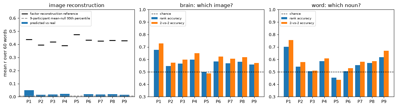
The table reports each held-out participant’s mean predicted-image correlation over 60 words, the factor reconstruction reference (factor ref r), and the decoding accuracies. The reference correlates the observed image with its reconstruction using that participant’s fitted factor weights. It describes representation of the observed image without predicting its weights from the noun embedding.

This reference is not an upper bound on correlation: ridge fitting and the decoding map optimize objectives different from Pearson correlation, so a prediction can have a larger correlation than the reference. It is also not a noise ceiling or a measure of repeat-to-repeat reliability.

t0 = time.perf_counter()
out = Parallel(n_jobs=3)(
    delayed(decode_participant)(s, E, Ws, Fs, imgs) for s in range(len(subjects))
)
S_brain, S_word, ceiling = (np.stack(x) for x in zip(*out, strict=True))
print(f"decoding time: {time.perf_counter() - t0:.0f} s")
recon_r = np.array([np.diag(S) for S in S_brain])  # (9, 60)
brain = np.array([scores(S) for S in S_brain])  # columns: top-1, rank, 2-vs-2
word = np.array([scores(S) for S in S_word])
print(
    "participant | recon r | factor ref r | brain rank | brain 2v2 | "
    "word top-1 | word rank | word 2v2"
)
for p in range(len(subjects)):
    print(
        f"P{p + 1:<10} | {recon_r[p].mean():7.3f} | {ceiling[p].mean():12.3f} | "
        f"{brain[p, 1]:10.3f} | {brain[p, 2]:9.3f} | {word[p, 0]:10.3f} | "
        f"{word[p, 1]:9.3f} | {word[p, 2]:8.3f}"
    )
print(
    f"{'mean':<11} | {recon_r.mean():7.3f} | {ceiling.mean():12.3f} | "
    f"{brain[:, 1].mean():10.3f} | {brain[:, 2].mean():9.3f} | "
    f"{word[:, 0].mean():10.3f} | {word[:, 1].mean():9.3f} | "
    f"{word[:, 2].mean():8.3f}"
)
print(
    "chance      |         |              |      0.500 |     0.500 |      "
    f"{1 / 60:.3f} |     0.500 |    0.500"
)

decoding time: 18 s
participant | recon r | factor ref r | brain rank | brain 2v2 | word top-1 | word rank | word 2v2
P1          |   0.051 |        0.438 |      0.676 |     0.728 |      0.017 |     0.701 |    0.755
P2          |   0.014 |        0.395 |      0.547 |     0.572 |      0.000 |     0.543 |    0.579
P3          |   0.018 |        0.418 |      0.567 |     0.598 |      0.000 |     0.506 |    0.510
P4          |   0.021 |        0.391 |      0.597 |     0.649 |      0.000 |     0.585 |    0.609
P5          |   0.001 |        0.475 |      0.500 |     0.488 |      0.017 |     0.453 |    0.437
P6          |   0.019 |        0.432 |      0.582 |     0.623 |      0.017 |     0.505 |    0.529
P7          |   0.017 |        0.426 |      0.569 |     0.606 |      0.017 |     0.555 |    0.582
P8          |   0.020 |        0.430 |      0.580 |     0.618 |      0.083 |     0.571 |    0.585
P9          |   0.014 |        0.427 |      0.558 |     0.571 |      0.017 |     0.618 |    0.669
mean        |   0.019 |        0.426 |      0.575 |     0.606 |      0.019 |     0.560 |    0.584
chance      |         |              |      0.500 |     0.500 |      0.017 |     0.500 |    0.500

The table distinguishes predicted-image correlation, the factor reconstruction reference, candidate ranking, pairwise discrimination, and top-1 identification. These answer different questions: good rank accuracy need not imply accurate voxel values or reliable top-1 identification. Compare participants as well as the mean; the permutation test below evaluates the mean statistics against relabelled embeddings.

7. Permutation test

Each permutation assigns the 60 embeddings to the 60 nouns at random and reruns the whole procedure (both mappings, all 540 folds, the inner choice of the penalty). The statistic is the mean over the 9 participants; p = (1 + number of permutations at least as large) / (1 + N_PERMUTATIONS). With the default N_PERMUTATIONS = 20 the smallest possible p is 1/21 ≈ 0.048; setting it to 100 gives finer p-value resolution (smallest possible p 1/101 ≈ 0.010).

What is loaded. By default (RECOMPUTE_NULL = False) the cell loads a saved null for 20 or 100 permutations with htfa.datasets.fetch_tutorial_fit. It uses the saved fit (section 3) and saved embeddings (section 5), matching the inputs of the observed statistics above; the input hashes are checked before use. RECOMPUTE_NULL = True reruns the permutations. It is required when REFIT or RECOMPUTE_EMBEDDINGS is True, so that the observed statistics and the null come from the same fit and embeddings.

# Number of permutations: 20 by default (smallest possible p = 1/21);
# 100 reproduces the full analysis (smallest possible p = 1/101).
N_PERMUTATIONS = 20
# Recompute the null (True), or load the saved null for 20 or 100 permutations,
# computed with the saved fit and the saved embeddings (False, the default).
RECOMPUTE_NULL = False
names = [
    "recon r",
    "brain top-1",
    "brain rank",
    "brain 2v2",
    "word top-1",
    "word rank",
    "word 2v2",
]
seeds = 1000 + np.arange(N_PERMUTATIONS)


def permuted_means(seed):
    """Relabel the 60 embeddings at random and rerun the whole decoding."""
    E_perm = E[np.random.default_rng(seed).permutation(60)]
    res_p = [decode_participant(s, E_perm, Ws, Fs, imgs) for s in range(len(subjects))]
    b = np.array([scores(r[0]) for r in res_p]).mean(0)
    w = np.array([scores(r[1]) for r in res_p]).mean(0)
    recon = np.mean([np.diag(r[0]).mean() for r in res_p])
    return np.r_[recon, b, w]


if RECOMPUTE_NULL:
    t0 = time.perf_counter()
    null = np.array(Parallel(n_jobs=4)(delayed(permuted_means)(s) for s in seeds))
    print(f"permutation time: {time.perf_counter() - t0:.0f} s")
else:
    if REFIT or RECOMPUTE_EMBEDDINGS:
        raise RuntimeError(
            "the saved null was computed with the saved fit and the saved "
            "embeddings; set RECOMPUTE_NULL = True to compute it from the ones "
            "used here"
        )
    if N_PERMUTATIONS not in (20, 100):
        raise ValueError(
            "saved nulls exist for 20 and 100 permutations; set RECOMPUTE_NULL = True"
        )
    saved_null = htfa.datasets.fetch_tutorial_fit(f"mitchell2008_null_{N_PERMUTATIONS}")
    if str(saved_null["fit_sha256"]) != htfa.datasets.TUTORIAL_FITS[NAME][1]:
        raise RuntimeError("Saved permutation null does not match the registered fit")
    if (
        str(saved_null["embeddings_sha256_of_E"])
        != hashlib.sha256(E.tobytes()).hexdigest()
    ):
        raise RuntimeError("Saved permutation null does not match these embeddings")
    assert list(saved_null["statistics"]) == names
    assert np.array_equal(saved_null["seeds"], seeds)
    null = saved_null["null"]
    print(f"saved null: {N_PERMUTATIONS} permutations; input hashes verified")
observed = np.r_[recon_r.mean(), brain.mean(0), word.mean(0)]
print(f"{'statistic (mean of 9)':<22} observed  null mean  null 95th pct  p")
for k, name in enumerate(names):
    p = (1 + np.sum(null[:, k] >= observed[k])) / (1 + len(null))
    print(
        f"{name:<22} {observed[k]:8.3f}  {null[:, k].mean():9.3f}  "
        f"{np.percentile(null[:, k], 95):13.3f}  {p:.3f}"
    )

saved null: 20 permutations; input hashes verified
statistic (mean of 9)  observed  null mean  null 95th pct  p
recon r                   0.019     -0.001          0.007  0.048
brain top-1               0.031      0.014          0.021  0.048
brain rank                0.575      0.498          0.528  0.048
brain 2v2                 0.606      0.493          0.531  0.048
word top-1                0.019      0.013          0.021  0.238
word rank                 0.560      0.497          0.517  0.048
word 2v2                  0.584      0.494          0.521  0.048

Use the observed statistics, null percentiles and p-values above to evaluate each metric separately. With 20 permutations, p-values cannot be smaller than 1/21. The 100-permutation asset provides finer resolution; neither setting makes these seven exploratory metrics a multiplicity-corrected family of tests.

8. Figures

For each participant, bars show mean predicted-image correlation and black ticks show the factor reconstruction reference. The dashed line is the 95th percentile of the permutation null for the mean across all nine participants. It provides context for the group mean; it is not a participant-specific significance threshold. The other panels show rank and 2-vs-2 accuracy in both decoding directions; top-1 accuracy appears in the table.

labels = [f"P{p}" for p in range(1, 10)]
x = np.arange(9)
fig, ax = plt.subplots(1, 3, figsize=(13, 3.6))
ax[0].bar(x, recon_r.mean(1), color="tab:blue", label="predicted vs real")
ax[0].plot(
    x, ceiling.mean(1), "k_", ms=14, mew=2, label="factor reconstruction reference"
)
ax[0].axhline(
    np.percentile(null[:, 0], 95),
    color="gray",
    ls="--",
    label="9-participant mean-null 95th percentile",
)
ax[0].set(ylabel="mean r over 60 words", title="image reconstruction")
panels = ((ax[1], brain, "brain: which image?"), (ax[2], word, "word: which noun?"))
for a, M, title in panels:
    a.bar(x - 0.2, M[:, 1], 0.4, label="rank accuracy")
    a.bar(x + 0.2, M[:, 2], 0.4, label="2-vs-2 accuracy")
    a.axhline(0.5, color="k", ls="--", lw=1, label="chance")
    a.set(ylim=(0.3, 1), title=title)
for a in ax:
    a.set_xticks(x, labels)
    a.legend(fontsize=7, loc="upper left")
ax[0].set_ylim(0, max(ceiling.mean(1).max(), recon_r.mean(1).max()) * 1.4)
plt.tight_layout()
plt.show()

Ranks of the true item among the 60 candidates over all 540 held-out words; under chance they are uniform. The plot and printed summaries show whether the true item tends to rank near the top and how often it appears among the best five candidates.

def true_ranks(S):
    """Rank of the true item among the 60 candidates (1 = best), per held-out word."""
    return np.array([1 + np.sum(np.delete(row, i) > row[i]) for i, row in enumerate(S)])


ranks_b = np.concatenate([true_ranks(S) for S in S_brain])
ranks_w = np.concatenate([true_ranks(S) for S in S_word])
fig, ax = plt.subplots(1, 2, figsize=(10, 3), sharey=True)
bins = np.arange(0.5, 61.5, 3)
for a, r, title in (
    (ax[0], ranks_b, "brain: rank of the real image"),
    (ax[1], ranks_w, "word: rank of the real noun"),
):
    a.hist(r, bins=bins, color="tab:blue")
    a.axhline(len(r) / 20, color="k", ls="--", lw=1, label="uniform (chance)")
    a.set(xlabel="rank among 60 (1 = best)", title=title)
ax[0].set_ylabel("held-out words (9 x 60)")
ax[0].legend()
plt.tight_layout()
plt.show()
print(
    f"median rank: brain {np.median(ranks_b):.0f}, word {np.median(ranks_w):.0f} "
    "(chance 30.5)"
)
print(
    f"rank 1: brain {np.mean(ranks_b == 1):.3f}, word {np.mean(ranks_w == 1):.3f}; "
    f"rank <= 5: brain {np.mean(ranks_b <= 5):.3f}, word {np.mean(ranks_w <= 5):.3f}"
)

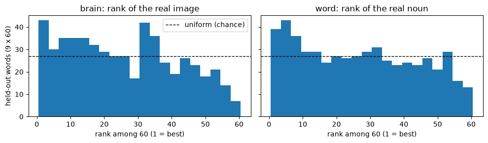
median rank: brain 25, word 26 (chance 30.5)
rank 1: brain 0.031, word 0.019; rank <= 5: brain 0.120, word 0.119

Illustrative held-out predictions for four nouns in participant P1 (hammer, house, dog, and car); these items provide concrete views of the prediction and reconstruction procedures. Each image is the deviation from P1’s mean image over the 59 training words, z-scored across voxels and drawn on the same color scale (±3; |z| < 1 not drawn).

Left: the real image (mean of 6 presentations). Middle (F w): the same image represented by the 100 factors with P1’s real weights. Right: the image predicted from the noun’s embedding by the mapping learned on the other 8 participants. The predictions are smooth because they are sums of 100 broad factors; the measured single-word images contain finer spatial variation. This display alone does not separate reliable detail from noise.

s = 0  # P1
examples = ["hammer", "house", "dog", "car"]  # illustrative nouns
z = lambda v: (v - v.mean()) / v.std()  # noqa: E731
fig, axes = plt.subplots(len(examples), 3, figsize=(15, 2.2 * len(examples)))
for row, w in zip(axes, examples, strict=True):
    i = int(np.flatnonzero(vocab == w)[0])
    keep = np.arange(60) != i
    real = imgs[s][i] - imgs[s][keep].mean(0)
    # rerun the word-i fold of participant s to get its predicted image
    train = [t for t in range(9) if t != s]
    Z = np.stack(
        [(Ws[t][keep] - Ws[t][keep].mean(0)) / Ws[t][keep].std(0) for t in train]
    )
    w_hat, _ = ridge_cv_predict(
        E[keep], Z.mean(0), np.arange(59), E[i : i + 1], ALPHAS / 8
    )
    pred = Fs[s] @ (w_hat[0] * Ws[s][keep].std(0))
    r = np.corrcoef(pred, real)[0, 1]
    assert np.isclose(r, S_brain[s, i, i])
    in_factors = Fs[s] @ (Ws[s][i] - Ws[s][keep].mean(0))  # real weights, F w
    r_f = np.corrcoef(in_factors, real)[0, 1]
    panels = (
        (row[0], real, f"{w}: real"),
        (row[1], in_factors, f"F w, r = {r_f:.2f}"),
        (row[2], pred, f"predicted, r = {r:.2f}"),
    )
    for a, v, t in panels:
        plotting.plot_glass_brain(
            to_nifti(z(v), s),
            axes=a,
            display_mode="lyrz",
            plot_abs=False,
            cmap="RdBu_r",
            vmax=3,
            threshold=1.0,
            colorbar=False,
            title=t,
        )
plt.show()
print("z-scored images, |z| < 1 not drawn, color scale -3 (blue) to +3 (red)")

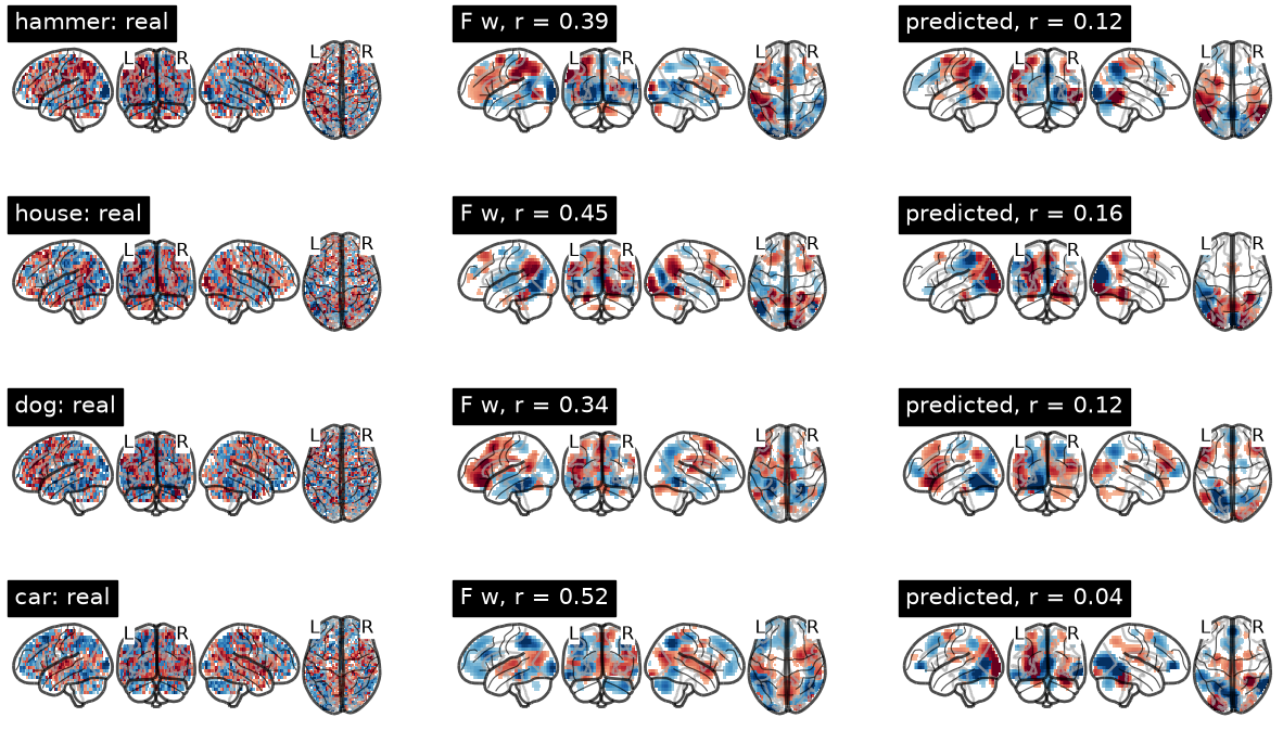
z-scored images, |z| < 1 not drawn, color scale -3 (blue) to +3 (red)

Summary

HTFA represents each participant’s voxel images using K=100 shared-factor coordinates. The two decoding directions test prediction of brain images from embeddings and identification of nouns from brain activity. Inspect the observed/null table and participant-level results before drawing conclusions about either direction.

The template and voxel standardization use all participants’ unlabelled images. The supervised mappings exclude the target participant and target noun, but this is not a fully inductive test of a template learned without the held-out data. The permutation test conditions on the fitted representation and saved embeddings. All cached nulls are checked against their exact fit and embedding hashes.

print(f"notebook run time: {time.perf_counter() - t_notebook:.0f} s")

notebook run time: 25 s